The normal loss when pre-training a language model is Cross-Entropy, which sounds more complicated than it is. As it generates a token, the model doesn’t just predict a token, it predicts a probability distribution across all possible tokens. Cross Entropy loss is -log(probability of the correct token) from that distribution.
If p(correct) = 0.99 → CE ≈ 0.01
If p(correct) = 0.5 (unsure between two tokens) → CE ≈ 0.693
If p(correct) = 1/100_000 (e.g. guessing uniformly) → CE ≈ 11.5
If you average the CE over a whole bunch of tokens (say in your validation set) and take e^(ave CE), you get the perplexity, or PPL.
The number gives you an idea of how many choices the model was considering. Perplexity of 1 means the model was always 100% sure and 100% right (a feat only Elon can achieve). PPL 2 means the model was flipping a coin between two tokens most of the time. PPL 50 means the model was uncertain between 50 plausible next tokens. Because you’re already calculating the loss, PPL is very cheap to compute, so it gets used a lot.
Prior to pre-training you’ll typically run a sweep of experiments of different architecture tweaks, and see which lower perplexity. During pre-training you’ll want to check whether the model is successfully learning, whether you should nuke a run rather than continuing: improvements in perplexity are a good guide to that. You can also score perplexity on fresh data using a well-trained model: data with a surprisingly high perplexity might be garbage, or a counting subreddit.
Still, you can have too much of a good thing. A new paper from Veličković et al “Perplexity cannot always tell right from wrong”, makes the argument that, much like with humans, its very easy to select for confidently wrong rather than uncertainly right.
We prove that, for a wide class of decoder-only Transformer-based language models, should the model be highly confident and correct on a sufficiently long input sequence, this must imply existence of another input where the model’s prediction is wrong, yet the log-perplexity of that prediction approaches *zero*
The basic idea is that when the model is confident, you can construct a different sequence that the model would be equally confident on but also… wrong.
This particularly shows up when contexts get longer, because all tokens are not equal. To give a trivial example:
In the word "strawberry," there are 8 Rs.
This is correct for every single token, except ‘8’. A highly confident model may have a lower perplexity for that sequence, as a whole, than a more correct but less confident one.
The current vibes in software engineering are a mix of crushing despair at years of accumulated personal skills being displaced by the CEO prompting some stuff, and crushing despair at years of corporate investment in an existing codebase that isn’t vibe-y enough. People worry whether the models will be effective in their programming language of choice, not on some general benchmarks.
One angle to approach that is to ask how well the language is covered by the distribution of the training data1. An interesting paper the other day gave a pretty clear idea of how to check: 1-shot some prompts against the base model and see if they ever get it right. Getting access to base models is not always possible, but you can certainly call the post-trained models with roughly the same idea: no tools, no iterations, just generate this program.
To try this, I2 wrote up 20 project-euler like3 puzzles of varying difficulties and had a few different models YOLO solutions in several languages. These ranged from common ones like Python to fairly rare ones like Zig and Hack.
After validating all the solutions, we can calculate some stats using pass@k: in k trials, how often did the model solve the problem. Here’s some stats for pass@1: what % of the time can you expect the model to one-shot the solution:
Lang
GPT-4.1 Mini
Gemini 3 Flash
OLMo 3.1
Kimi K2.5
GLM-5
Python
.93
.99
.72
.97
.98
Type Script
.94
1.00
.43
.95
.95
Go
.95
.91
.46
.86
.86
Rust
.89
.94
.43
.95
.95
Kotlin
.90
.99
.29
.91
.93
OCaml
.76
.86
.08
.94
.90
Zig
.14
.55
.00
.79
.88
Hack
.43
.76
.05
.47
.68
And here is the same thing for pass@128: what is the chance it is right at least once in 128 samples:
Lang
GPT-4.1 Mini
Gemini 3 Flash
OLMo 3.1
Kimi K2.5
GLM-5
Python
1.00
1.00
.95
1.00
1.00
Type Script
1.00
1.00
.90
1.00
1.00
Go
1.00
1.00
.85
1.00
1.00
Rust
.95
1.00
.88
1.00
1.00
Kotlin
1.00
1.00
.59
1.00
1.00
OCaml
.98
1.00
.38
1.00
1.00
Zig
.49
1.00
.05
1.00
1.00
Hack
.99
1.00
.46
1.00
1.00
To make that a bit more visual, here is a per-language chart for GPT-4.1-mini:
Given enough chances GPT 4.1-mini solves all the problems, in almost all the languages. Of course, we don’t actually know what GPT 4 was trained on, but we do know what OlMo 3.1 was trained on, thanks to the wonderful folks at AI2. That means we can see how much code-specific data for each language there was4:
Language
Code Corpus (GB)
Est. Tokens (B)
Category
Python
60.40
17.3
High-resource
TypeScript
26.52
7.6
High-resource
Go
23.78
6.8
High-resource
Rust
9.11
2.6
Medium-resource
Kotlin
5.68
1.6
Medium-resource
OCaml
1.03
0.29
Low-resource
Zig
0.18
0.05
Low-resource
Hack
0.00
0.00
Very-low-resource
There is a pretty decent correlation between the presence of training data and the pass@k rates. But, importantly, its not 1: despite Hack having no StarCoder data and Zig negligible, the model clearly does know at least something about them. Given enough chances it has a decent chance at coming up with the correct answer for Hack, and a non-zero one for Zig:
We have seen for human language that models learn a language substrate, enabling them to perform strongly even on tasks they haven’t seen such as translating between unseen language pairs. I suspect something similar happens with code: despite the language differences there is a logical programming substrate, and the model doesn’t need much exposure to the language in order to generalize to it.
Once you start giving the model multiple attempts, it gets into the right region quickly for the high-resource languages: with GPT-4.1 mini, Python, TypeScript, Go and Kotlin saturate at k=10. The less-common languages continue to rise: the model can write valid OCaml or Zig or Hack but need more attempts to stumble into the right region.
Thinking models flatten the curve substantially. Kimi K2.5 and GLM 5 both use high effort by default5, and that appears to give them multiple bites at the apple from internally exploring and self-correcting. By k=10 the models saturate all problems on all languages, though at the cost of a remarkable number of tokens6!
It’s also instructive to see the ways in the which the models get it wrong. There were four patterns that showed up:
Ecosystem: One problem involved a sum of very large digits. GPT-4.1 Mini regularly used num::BigUint. This is a crate, not a standard language feature, and in an agentic loop would probably be a very valid choice but doesn’t strictly work. In contrast, GLM-5, a thinking model, implements digit-by-digit multiplication from scratch with Vec<u32>.
API confusion: The model knows roughly what the code should look like, but chooses the wrong API. For example, OlMo generated while ... do ... in mixing OCaml’s while...do...done loop with Haskell’s do notation and OCaml’s let...in binding.
Surface-form invention: The model has a sense of how things stylistically look in the language, but doesn’t know the real API. GLM occasionally writes Zig with invented functions: std.mem.Allocator.alloc(usize, limit) (Allocator is a type, not a callable) or @intCast(usize, limit), which actually was valid syntax in earlier versions.
Systematic convention gaps: Models would regularly put in <?hh for the hack samples, which broke in modern Hack.
My takeaway from this is that models learn to code, not just to reproduce syntax. That means you can almost certainly post-train or prompt your way out of most programming language problems with any frontier model: while some models were still pretty poor at Zig even with a lot of tries, Gemini most certainly was not. I doubt the folks at GDM spent a whole lot of time on Zig evals7.
A well pre-trained model has broad capabilities in programming, and it’s mostly a case of eliciting them rather than having to teach them.
I’m going to take as a given that models are good at generalizing within the distribution of their training data, and poor at generalizing outside it. This is not settled! Reasonable people can disagree! But, it’s a decent starting point. ↩︎
Not actually project Euler. I confirmed that the models never respond with an actual Euler puzzle answer in the incorrect ones, so I’m fairly (this is not good science) sure it wasn’t memorization. ↩︎
OLMo’s full training corpus (Dolma v1.7) includes a massive web crawl in addition to code-specific data from StarCoder, so the 0.00 GB for Hack means “absent from code specific training ” not “absent from all training data”. Hack documentation and other content are almost certainly present in the web crawl portion. ↩︎
Gemini also reasons, but the 2.5 Flash model was doing minimal reasoning when answering. ↩︎
Somehow averaging over 3k per sample for GLM, I say while ruefully staring at my OpenRouter bill. ↩︎
By posting this on the internet I am guaranteed to be corrected, at length, by a Googler ↩︎
There are a lot of things folks do on GPUs (including, sometimes, graphics) so I have an approximately-correct taxonomy of operations to group them in to:
Dense compute: A matmul or a convolution.
Map: Elementwise/pointwise work on each value of a tensor.
Reduce: Process a tensor into fewer dimension, like a sum.
Transforms: Change data structure. Easy ones like transpose, annoying ones like scatter/gather.
Synchronize / Communicate: Move data, or wait for it (copies, collectives, fences/barriers).
At the moment people are pouring billions of dollars into hardware that primarily does 1. And, at the same time, many of the greatest minds of our generation are attempting to ensure that the hardware spends as much time doing 1 as possible.
The biggest barrier to doing a lot of dense compute is 5: moving things in and out of memory. Launching kernels, transferring data between host and device (or between devices), moving data between global memory and registers and so on. It’s like there’s a box defined by Data × Footprint1 × Time, and everyone is trying to keep it as full as possible.
This involves tradeoffs. You want to mul as many mats as you can, but you only have so much room to store accumulators. Fetching new data from memory also takes a while. You can keep many in-flight fetches around, but each one expands the kernel Footprint, lowering occupancy.
There are 3 tricks that we can use to help fill up the box by stitching different operations together:
Epilogue fusion: take an elementwise op and fuse it onto the end of a dense op, so that when the MMA produces output, the elementwise op can be run while the output data is still in registers. A classic example: fuse the activation after the dense compute in a feed-forward net.
Vertical fusion: take two subsequent operations and chain them together to avoid running a loop for one, writing it back, then running a loop for the other2. A classic example is Fused LayerNorm: normally you’d need to add elements, then collect stats for the normalization. You can fuse the two to collect the stats as you add the residual.
Horizontal fusion: doing different things over the same data, in parallel. The Q, K, and V projections in a transformer all need the exact same input, so are good candidates to fuse horizontally.
You rely on the design of the hardware to enable some of this. For example, an epilogue fusion is beneficial because it’s one kernel launch instead of two, and because the work doesn’t need to be written back to global memory, but also because the epilogue can overlap with other work.
It’s not always obvious how to put these fusions together. Flash Attention was such a breakthrough because it made dense op fusion possible. The naive attention block has a softmax in the middle: Softmax(QK^T / √d) · V. That softmax is a reduction op, which means it needs all of QK^T to be computed first, a pretty large matrix. Tri Dao and colleagues realized that if you used online softmax you could calculate the softmax for subsets of the QK matrix, and avoid materializing the whole thing. They enabled fusing the QK into the softmax and the V in one kernel, at the tile level.
Tiles are the subsection of a matrix you’re working on at any given time. In a matmul, tiles from both input matrices are loaded and multiplied, to produce an output tile. There’s a useful image of this in the Nvidia blog post on cuTile, Nvidia’s most recent entrant into the the kernel-development landscape. To side-step concerns of plagiarism, I had nanobanana plagiarize it for me:
cuTile is built on a well-specified intermediate representation called TileIR. There’s an experimental backend for Triton that lowers to TileIR too. While Triton is block-oriented rather than tile-oriented, in practice what you mostly work on in a thread-block is… a tile. TileIR elevates the tile to a first-class concept.
You can see this by generating the same kernel against the regular backend and the TileIR backend. Triton’s intermediate representation (TTIR) uses pointer arithmetic: generating offsets, computing masks, loading from explicit addresses. Here’s a bit of an inner loop of a matmul. It groups up which data it wants, loads the tiles a and b by pointer, and computes the dot product:
TileIR on the other hand preserves the tile as a semantic object. This snippetis doing exactly the same thing, but this representation elides the pointer math and masking:
This is a nice IR (compact!), but from my perspective the most interesting part is that load function: tile_load_token_ordered.
The “time” dimension of the Data × Footprint × Time box is the hardest one to manage. Time questions separate performant kernels from slow ones: When to prefetch, how to overlap loads, and so on. Since the advent of warp specialization, the Triton compiler has been exploring pipelining options through heuristics and autotuning, and kernel engineers have been going straight to the hardware with explicit barrier API extensions like TLX3 and Gluon4 .
TileIR goes a somewhat different route. It assumes an unordered memory model: the order your code is written in does not determine when data is actually available. Instead, each memory operation returns a token and you attach semantics to it: read-only, write-only, read-write and so on.
By being explicit about memory dependencies you give the compiler freedom to manage the Time dimension. Where accesses don’t overlap the compiler can freely reorder them. Where they do, the token chain tells the compiler exactly what depends on what. The kernel expresses intent; the compiler maps that to the hardware.
TileIR is (mostly) targeting Blackwell right now, and the experimental backend is still early. The open question is whether we can express this smoothly enough in the syntax of kernels to actually enable taking the same kernel across hardware, or whether we are just adding some syntactic-sugar to avoid when doing hardware-specific tuning.
That said, the idea feels pretty right? The tile is the unit with which we can express what we actually mean about memory, ordering, and fusion. The CUDA programming model was always about bounded-linearity within a massively parallel framework, and this loosens the bounds that little bit more.
Use of available registers and shared memory, for example ↩︎
This is loop fusion, in compiler terms. There are other things you can do, but this is the big one. ↩︎
Triton Language Extensions, from Meta. As a disclaimer, these are the folks I work with. ↩︎
One of the persistent questions in model development is whether reasoning actually involves… reasoning. As in: are we seeing actual logical conclusions, or just better recall of knowledge and patterns from the training set? LLMs are trained on, roughly, the web, which makes answering that question tricky: almost everything shows up in some form. A model that appears to “reason” through a physics problem could just be pattern-matching an irritated Reddit reply it saw during training.
To this end, we build a fully controlled framework that isolates the contributions of each training stage. Our design is based on three principles: (i) fully controllable synthetic reasoning tasks with explicit atomic operations and DAG-defined dependency structure; (ii) observable, parseable reasoning processes enabling process-level evaluation and reducing reward or evaluation hacking; and (iii) systematic manipulation of pre-/mid-/post-training distributions to attribute causal effects to each stage.
The authors break the problem of reasoning and training data down along two dimensions.
1) Breadth-wise: can the model generalize from one type of problem to another (structurally similar) one in a different domain? 2) Depth-wise: can the model reason correctly for longer, and hence solve harder problems?
Rather than train on the internet, they build synthetic Math-puzzle reasoning tasks using a dependency-graph framework inspired by GSM-Infinite. By varying the depth of the reasoning chains required, and by generating structurally equivalent tasks across different domains, they try to tease apart those two aspects and investigate them separately.
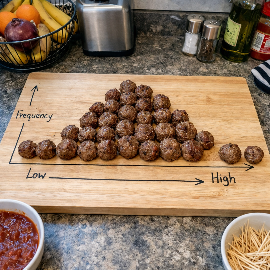
For the breadth side the model needs to generalize, to transfer learning across domains. The paper finds that the target domain has to be “in-distribution: the model has to have some examples in the pretraining set. They test this by using pass@128: if you give the pre-trained model 128 attempts, does it get the answer right even once? If so, you can use reinforcement learning or SFT to help the model get reliably better.
It’s a bit like having studied Spanish at some point and forgotten albóndigas, the word for meatballs. If, for dietary preference reasons, you came to use that word regularly it would likely lodge itself in your brain more easily and you’d go from a lowish chance of getting it right to a much higher one.
The paper is saying you must have this baseline in their to amplify with RL. Daniel Han of Unsloth describes this by saying with RL “luck is all you need”. If the model never gets the answer right, there is nothing much to reinforce (and you are stuck with paella).
Depth on the other hand does seem to something we can kinda make up in post-training. Even if a model has only been pre-trained on problems up to a certain complexity, post-training on harder problems consistently enables it to solve them. The model is able to compose more complex patterns based on the simpler ones in its training set1. To continued our tortured analogy, this is more like being reminded of several Spanish words and, over time, learning to stick them together into actual sentences.
Practically this means your pre-training data is a bet on what the model will ever be able to reason about, and post-training refines how well and how hard it can think within those domains.
That approach also gives a useful tool for identifying whether something is in-distribution. If you want to know whether a model can learn a new capability through post-training, check pass@128 first. If it never gets the answer right in 128 attempts, you probably have a pre-training gap, not an RL problem.
The paper also spends a while justifying curriculum training, giving the model problems just on the edge of its capabilities before introducing harder ones. Recent work from the FAIR Paris folks and others show you can somewhat automate this by generating problems from the same model you are training! ↩︎
Every big software engineering team right now is racing to out-do themselves on their adoption of agentic coding practices, and ship faster. There is something more insidious going on with many of the software engineers I talk to1 though. A lot of pressure to build “more! faster!” comes from themselves.
This shows up all over: the “you only have 2 years to escape the permanent underclass” meme2, or the various breathless LinkedIn or Twitter posts of 996’ing startups, labs, or particularly obsessive interns.
Things that used to require teams can now be done by a sufficiently keen solo engineer with a gang of Claudes, or Codexes, or a K2 agentic-swarms. That is thrilling, and it opens up the door to projects that you wouldn’t normally have bothered building. But it also open the door to thinking you need to build those things, and that’s not quite the same.
One of the observations of most people that take an extended leave from a large corporation is that much of the work they were doing wasn’t all that important. Either no one did it while they were out, or how they left it was… fine. Yet, much of that work somehow regains urgency as they come back to the role.
It’s very hard to tease apart how much of your output actually matters. Coordinating a large group of people inevitably takes overhead, and so many annoying aspects of work are genuinely important. But, much like Wanamaker’s famous quote about advertising, half of the work you do doesn’t matter, the trouble is you don’t know which half.
Adding a helpful and harmless model to the mix can certainly accelerate the rate of output, but it doesn’t do much about determining which bucket the work goes into. In fact, I’d say that the problems you take on when given a Max subscription are mildly more likely to to be things that haven’t been done because they are not worth doing. The combination of increased capacity and a pervasive sense of urgency is not a great recipe for quality decision making, or for a healthy relationship with your work.
It can be helpful to take the outsider perspective, at work or with personal projects. Would ask you someone else to do whatever you are considering, even with the expectation they would leverage agents to help them?
It’s often easier to see the value in something, or lack thereof, if you have to convince someone else of it. That can save you from some rabbit-holes filled with a sense of obligation to “extract value” from the time you already sunk into a misguided project.
This doesn’t mean you should ignore all of the ideas you have: you really can just do things, and you sometimes should! Just be clear about whether you want to spend your time3 that way, regardless of what the agent is doing.
When I was writing recently about MoEs I was focused mostly on the architectural reasons that we use them. One thing I hadn’t considered is that they might actually be better at learning as well.
Our findings reveal that MoE architectures form a low entropy backbone of consistently reinforced neurons, which leads to an early consolidation of their importance profiles and, in turn, underpins their functional robustness. This resilience, stemming from more distributed knowledge storage, contrasts with the greater brittleness and knowledge concentration in the dense model. These phenomena collectively demonstrate that architectural sparsity is not merely a computational shortcut but also acts as a useful inductive bias that fosters stable and robust learning
To land that somewhere between academic prose and GPT-speak1 the results of the paper are suggesting that MoEs learn more effectively, and store their core knowledge more robustly.
They measure this with Log-Probability Increase (LPI), which lets you estimate how much each column in the output projection for a layer in the model contributes to the final score. It gives you a sense of how much smarter the model gets from that specific chunk of the weights2. They track this “neuron importance” measure over multiple checkpoints using the (very!) open models from AI2, OLMo-7B and OLMoE-1B-7B.
In the MoE the set of important weights is both more stable and stabilizes earlier in training: the model develops a core of understanding and builds on that. This might mean MoE training is genuinely more effective than dense. The dense model is regularly thrashing its core understanding as updates come in, while the MoE protects it and lets the model focus more on nuance.
Or! It might be entirely an artifact of model differences. As the authors note the two models are quite different: different training data sets, different lengths of training, and different depths (16 vs 32 layers), as well as, you know, being an MoE or not. Finally, the actual LPI version they use3, Gated-LPI, bakes in the MoE routing. It’s not totally clear whether we are seeing “neurons that matter”, or mostly seeing “routing patterns that matter”.
I do think4 this is likely showing something interesting, even with some skepticism. The “smearing” of knowledge across weights is how I described what we are trying to avoid with MoEs, and it may be useful to have a more mechanistic understanding of how that actually happens. The authors observe that the stability curve rises, drops and consolidates. Even if this is just an artifact of routing, it’s quite possible there is a critical phase in the training where that routing locks-in.
If that idea is right, we might already be shaping that phase. The load-balancing tricks that made MoEs practical could be doing double duty as scaffolds for learning.
Sparsity is not just a shortcut — it’s crucial to learning ↩︎
For a given prompt. They actually use some fairly advanced evals for this, rather than the general basic benchmarks ↩︎
And created, to make it plausible to do this work! ↩︎
Do not draw any research conclusions based on this website ↩︎
In the heady world of AI progress, context lengths have seen somewhat more languid growth. After rapid progress up to the 100-300k token range, they’ve largely stayed there for frontier models. We now have a couple of 1m token models that appear economically viable1, with Gemini and Sonnet, but Opus 4.5 (for example) stuck with the 200k window of its predecessor.
The fundamental challenge with long contexts is the interaction between tokens, particularly in the prefill (prompt processing) phase where you have to do this for a whole lot of tokens at once before you can generate anything.
For each token attention calculates:
1) The key: when to use this token 2) The value: what information this token contributes 3) A query: what each token is looking for
Each2 token’s query is compared against prior tokens’ keys to get weighted scores; the resulting weights mix those tokens’ values.
Then, in decoding you make this calculation repeatedly. The 500th token has a new Key, Value and Query, but the 1st token has the same.
It turns out you can save yourself a lot of work by just keeping around the Keys and Values from the previous generation and loading it in for the prior tokens. Then you just have to update for the newly added token. This happens for every layer in the model, so it’s a significant amount of computation saved.
Of course, you have to stick that cached copy somewhere. Because it’s used in each round of generation it needs to be rapidly available, to avoid adding a bunch of latency. In practicality that means it has to be in the high bandwidth memory, which is a scarce resource. So the longer the context the more memory you need to hold it, and the more memory you need for a bigger cache.
Larger context windows have been unlocked in large part by more memory on the card and in a somewhat smaller part by more rapid scale-out interconnect like NVlink3.
Meanwhile, here’s Uncle Jensen at CES, via Stratchery‘s excellent analysis of the announcements:
this context memory, which started out fitting inside an HBM, is no longer large enough. Last year we created Grace Blackwell’s very fast memory, we call fast context memory. That’s the reason why we connected Grace directly to Hopper. That’s why we connected Grace directly to Blackwell, so that we can expand the context memory. But even that is not enough, and so the next solution, of course, is to go off onto the network, the north-south network, off to the storage of the company. But if you have a whole lot of AIs running at the same time, that network is no longer going to be fast enough. So the answer is very clearly to do it different, and so we created Bluefield-4 so that we could essentially have a very fast KV cache context memory store right in the rack.
It’s quite possible this kind of in-rack memory will unlock significantly larger context windows. I do wonder what this will mean for actually using long-context models. Dealing with multiple-million tokens of context is still going to take a bit of time to process. For the kind of interactive use cases that have worked best with LLMs (Claude Code, Computer Use, Cowork etc.) I suspect latency will be a bit of a pain point.
What is kind of interesting is that all the providers at this point have some form of prompt caching option. Most of the time with a KV cache you build it up as you go, but in some cases you are going to actually generate the exact same cache in multiple different sessions. A good example would be a long system prompt: you can generate the KV cache for that, stick it on slower memory4 and then load it in to HBM for a new session. This can save a bunch of compute, and is very practical for a lot of use cases.
One interesting thing this might do is enable “whole codebase” type queries: the vast majority of assets (e.g. code) in a given work session won’t change, so you could cache the KV for everything, and have it in context for later use
I’m hopeful that as Blackwell, TPUv7 and MI450 come online we will see context lengths unstick and move up, and perhaps with Vera Rubin we will really get rid of “compacting” for some practical set of cases.
So many asterisks should go here after this flagrant assertion ↩︎
Technically in most cases this is between each token’s Query and the Keys of the tokens before it, thanks to causal masking ↩︎
You have to do some work to distribute things of course, but if your model is multi-card anyway, then you can distribute the KV cache fairly easily. TPUs have chonky scale-out bandwidth, probably one of the reasons Google was able to offer 1M first. ↩︎
For clarity, this might not actually be how its implemented at Throppy/Google/OAI, they might just keep it in HBM anyway. But it feels like you could do that? ↩︎
There are two really good ways to learn the deep fundamentals of a field. One we could call the Carmack/Ilya method: get an expert to give you a list of the seminal papers, systematically work through them, and in the process develop a deep, grounded intuition. This seems to work. The second is: funny tweets.
A case in point:
ok so: engram is moe over ngramed memory mHC is moe over the residual stream NSA is moe over attention MoE is moe over FFNs … im sensing a theme ….
Other than the fact you have to be in a very particular niche in order to understand all the acronyms in that tweet, the idea that everything is an MoE feels right? Pretty much every notable model release, and probably all the secret frontier models, are MoE.
Like every other idea in deep learning this goes back to something Hinton did in the 90s, specifically the paper Adaptive Mixtures of Local Experts by Jacobs, Jordan, Nowland and Hinton:
If backpropagation is used to train a single, multilayer network to perform different subtasks on different occasions, there will generally be strong interference effects that lead to slow learning and poor generalization. If we know in advance that a set of training cases may be naturally divided into subsets that correspond to distinct subtasks, interference can be reduced by using a system composed of several different “expert” networks plus a gating network that decides which of the experts should be used for each training case. […] The idea behind such a system is that the gating network allocates a new case to one or a few experts, and, if the output is incorrect, the weight changes are localized to these experts (and the gating network).
The idea is that if your data naturally clusters, then having separate networks avoids smearing understanding across the weights. A dataset with both German and English training data might produce a model that mixes up both languages. If we train two different experts and learn a gating network, we can get a clean “German-speaking” model, and a clean “English-speaking” model, in one.
Also, like every other idea in deep learning, this was very clever, but painful to train. In particular, this was because the decision about which expert to choose was a bit of a cliff. If you choose the German expert when you needed the English expert then the German expert would get some loss, but the English expert would get none. This could lead to the awkward situation where the German expert performed better for both English and German: you ended up with a smaller, smeared model, and a dead expert.
Noam Shazeer and co came to the rescue in 2017 with the excellently titled “Outrageously Large Neural Networks”. They introduced concepts that didn’t fundamentally change the approach, but did make it practical.
The key trick was adding an auxiliary loss that penalized the model for using one expert over the others. By adding some noise to the gating decision they helped it be differentiable and ensure errors could flow back effectively. This gave the training process a much better chance of avoiding this kind of “winner-takes-all” collapse.
Over time these methods were refined. In a contemporary MoE like DeepSeek v3, sigmoid-based routing removed the noise from the gating and the auxiliary loss is replaced in favor of a what they call bias updates: they just put their thumb on the scale during training if some experts aren’t getting enough samples, which seems to work great.
All of that is about how we got MoEs to scale, but doesn’t really say… why? Intuitively, if you can train a model with X parameters, it seems like it would be better to have all of them doing something (a dense model), rather than some subset1?
The main reason this has taken over the field is it is a way of decoupling capacity (how much can the network “know”) from compute (how much work does it do for each input).
In a dense model when you add a new token to train you send it to all parts of the model: every bit of capacity touches it, each of which uses some compute to process. MoEs are a form of sparsity: a way of ignoring some of the parameters. They let you add capacity without adding compute2.
There are other ways of achieving the same result, but the MoE approach is very hardware friendly. You’re still mostly doing dense matmuls, just split between experts. In parallelism terms, Expert Parallelism is efficient because you’re moving tokens between devices: it needs an all-to-all, but the data volumes are manageable.
The tweet calls out NSA, engram and mHC, all recent papers from Deepseek. But underneath it calls out the design pattern: make a few alternative compute or memory paths, then use a learned gate to pick (or mix) a subset of them, per token. You get sparsity at the routing level, decoupling formerly coupled aspects, while each path can remain fairly dense and hardware-friendly.
Engrams makes the argument that language models have to do two things: reasoning and looking stuff up. The reasoning works great with stacks of Transformers, but the looking-stuff-up part is approximated through computation rather than just… looking stuff up.
This process essentially amounts to an expensive runtime reconstruction of a static lookup table, wasting valuable sequential depth on trivial operations that could otherwise be allocated to higher-level reasoning.
Classically, Natural Language Processing used a lot of N-grams: representations of more than one token at a time, but language models pretty much dropped that in favor of a fixed vocabulary. Deepseek is bringing it back. These extra embeddings are retrieved for subsets3 of the tokens in the context window, the resulting vectors are summed4, then the model gates how much to incorporate the information based on the current state.
It’s the same move of decoupling compute and capacity. Here they are adding a bunch of extra storage parameters but letting the model learn whether or not to use them. Because the retrieval is based on tokens the table doesn’t have to live in VRAM but can be loaded with the input5 .
The second paper, Manifold-constrained Hyper Connectors is the most math-heavy of the recent release, and it builds on one of the most cited papers in ML: ResNet.
In the bad old days ,the “Deep” in Deep Neural Nets didn’t really exist: you could theorize, but if you tried to train one you’d get into a place where the early layers received basically no useful loss signal. ResNets fixed this in the simplest way possible: As well sending through the “output” of a layer, you sent through the input as well. This gave an efficient highway for loss gradients to flow back and enabled successfully training much, much deeper models.
mHC builds on an observation that ResNets hard-code another compute/capacity tradeoff: the size of the residual channel. If you think of a layer of a transformer: it has an input of C tokens, and an output the same size. The residual connection works by summing the input tokens and the output tokens. That’s assigning as much information capacity to the residual channel as you do to the processing channel. E.g.
Layer 0 gets raw tokens, and outputs a sum of raw+contextualized tokens
Layer 1 gets layer 0 tokens and outputs a sum of layer0+contextualized tokens
Etc.
At the end you get a cake recipe
But maybe that cake recipe would be better if Layer 2 had access not just to the layer0 tokens, but also to the raw tokens? We don’t really have a way to express that outside of adding extra skip connections. Hyper Connections widen the ResNet channel into multiple lanes, and mHC lets the model decide what to put in each: so you could have layer 1 putting layer0 context in one lane, and raw tokens in another lane6 . If MoE lets you take a bunch of parameters and selectively route tokens to a subset, then mHC lets you take a bunch of residual bandwidth and selectively mix the information flow from your module to a subset of it.
Finally, Native Sparse Attention follows the classic Deepseek move of throwing a bunch of engineering wins together. Instead of assuming the amount of attention compute for each token in is the same they are scaling it dynamically based on the content itself. They mix the outputs of a pooled version of the content window to get a compressed representation, a MoE-style gated selection from the full context window7, and a classic sliding window attention.
This is the pattern MoE exemplified:
look at what is constrained
add more of it, but make it conditional to avoid scaling other things at the same time
It’s a thread that runs through an awful lot of the industry right now. Understanding that is useful when anticipating where the things are going to go next.
Or, you could have saved yourself a lot of time and just liked the tweet.
MoEs do have some inference advantages: if you have a 100bn parameters model where just 20bn are active for a given token you simply have to do less work than a 100bn param dense model. That’s a win for latency! But, you still have to store all those 100bn parameters, meaning you need quite a lot of memory kicking around. ↩︎
More specifically, they make the ratio of adding capacity and adding capacity very flexible: modern MoEs often have many experts and activate several at a time. ↩︎
In practice they inject the ngram embeddings at a couple of different points later in the model, where empirically there seemed to be enough context for the model to make useful mixing decisions ↩︎
The specific clever thing the Deepseek folks added was a constraint to stop this from exploding, using the wonderfully named Sinkhorn-Knopp algorithm (apparently) ↩︎
Based on those pooled tokens. Effectively its taking the “summarized” context window, and using runtime gating to decide which bits of the context window to add in full. ↩︎
I think the most important AI question is, at some level, how do you deploy it so that it is a genuinely positive force across a wide spectrum of people.
I like to tell a story to describe Why Are Things This Way, for some wide hand wave of the world right now and it goes like this: The post-Cold War era marked a renaissance in global trade, what some people call the Pax Americana. This period of globalization rested on two American pillars and one Chinese: the U.S. dollar’s status as the world’s reserve currency, the U.S. Navy’s command of maritime shipping lanes and the rapid development of highly scaled manufacturing.
Underpinning this system was a constellation of technologies: containerization1, ERP systems, advanced telecommunications, the financialization of assets, and cheap energy. China’s accession to the WTO in 2001 was the culmination of its Reform and Opening policy, with leaders like Hu Jintao embodying a sense of forward momentum. We were at the apex of Francis Fukuyama’s “end of history”: the belief that liberal democratic capitalism represented the final stage of human political evolution.
This felt like a rising tide that might, for once, actually lift all boats. Growth did materialize. We witnessed a substantial economic expansion that lifted millions out of poverty, most dramatically in China but also across dozens of countries where GDP and living standards surged.
It was easy to look at this trend line and extrapolate upwards. The most common objection to that extrapolation was that it relied on non-renewable, extractive energy and materials 2. But I think this argument was a mistake on both sides: globalization represented a step change: a one-time shift enabled by a unique convergence of technologies that amplified the principles of specialization and trade to an unprecedented scale.
These technologies were big leaps, but their diffusion unfolded gradually, over decades. This extended rollout created an illusion of continuous growth. As Jeffrey Ding argues in his excellent 2024 book Technology and the Rise of Great Powers, the critical factor is not which nation invents technology first, but which spreads it through their economy faster. The same principle applies globally: diffusion creates the feeling of growth, but its just the future being unevenly distributed. We thought the end of the Cold War ended history, but in reality it just gave us a really good logistics stack.
The Great Financial Crisis of 2008 was the first major crack, exposing a disconnect between elite consensus and public experience. Contagion from the U.S. subprime mortgage market rippled worldwide, shattering faith in both institutions and experts. Austerity measures inflicted deep pain on the median voter, while ZIRP boosted GDP figures and asset valuations, widening the gap between elite enrichment and broad-based prosperity. COVID-19 extinguished any lingering illusion of elite competence. Chains collapsed across critical sectors from masks to electronics to, oddly, toilet paper.
Today, in the post-pandemic, post-austerity landscape, we’ve seen a decisive shift toward realpolitik and narrow, short-term domestic political calculation: people are less trusting of “the system” and more receptive to those actively disrupting it.
If you ask a random person in Hayes Valley they’ll say that AI is a similar step change, maybe even larger: it could lead to flourishing prosperity or possibly doom everyone to being consumed by a rogue instance of Claude obsessed with the Golden Gate bridge. Unlike the internet or mobile phones AI is emerging in a volatile, multilateral world with a broken trust environment.
AI needs vast resources: data, compute, electricity, technical skills, integration and political support. The US and China have adopted somewhat divergent approaches to how to manage that.
The U.S. model emphasizes corporate AI accountability and regulation that favors large incumbents, restriction over compute resources through export controls, and voluntary safety frameworks developed largely by industry. In essence, they are asking the public to trust corporate institutions to manage AI safely, and to deliver the long-term societal benefits to consumers. It’s downstream of the way the tech giants like Microsoft, Google and Apple have navigated government before: hands off during rapid growth, then clear regulations to offer a stable business environment.
China’s Internet companies are under no question of who is in charge, particularly after the crackdowns on gaming and social media a few years back. The Chinese Communist Party is caught in a bind: AI aligns very well with the kind of hard science, foundational technology they want to prioritize, but is dependent on foreign technology and needs the kinds of data and skills that exist within the big social conglomerates they just tried to reign in. China is running a playbook of rapid diffusion and explosive competition, with the government putting heavy hands on the scale: who can buy which GPUs, what kind of content controls must exist, and a national level AI plan. It says to the public: trust in the party, and we will ensure AI delivers social benefit, for our definition of “social benefit”
One major question, going into 2026, is which party will speak for the Americans who abhor the incursions of A.I. into their lives and want to see its reach restricted. Another is whether widespread public hostility to this technology even matters, given all the money behind it. We’ll soon start to find out not just how much A.I. is going to remake our democracy but also to what degree we still have one.
Goldberg is asking who will promise to assert state control for AI: who will bring the Chinese model to America. The fundamental problem for me is I’m not sure that the public trust the government much more than they do corporations, or the media.
If AI is a global-scale step change it requires global coordination, which is expensive: it’s something folks can engage with when everything is going well. When times are tougher, economic interdependence morphs into leverage for coercion and control. Blackwells and rare earths and SWIFT messages become chips on the bargaining table.
Billions of people use large language models, which gives the creators of those models influence in how people act. But thus far the influence on the models from their users is very indirect: aggregate usage patterns or occasional thumbs up/thumbs down feedback. Open Weight and Open Source models offered folks more control, but despite the slow death of scaling the ability to train and operate a true frontier model remains a very large hurdle.
What would it take for people to believe that this power is being used in a way that includes them, instead of being done to them? In a high-trust world you can do that with credentials and commitments. In this world you can’t. People don’t need safety and impact reports from labs or promises of benevolence from the state. They need leverage.
Trust can’t scale, but verification maybe can. That requires independent auditing, liability, and transparency around capabilities and how those capabilities are being deployed. Open weights help, competition helps, and national strategies help, but none solve the whole problem. We’re building machines that can reason. We also need to build systems where the people who own the machines can’t silently rewrite the terms of everyone else’s lives.
What we do in machine learnings owes a lot to the history of computer graphics. Folks like Kurt Akeley, one of the founders of SGI, identified that 3D graphics have a naturally pipelined structure. You have a high volume of similar operations, such as applying pixel-y soldier textures to a mesh of triangles, and by pipelining them you can find an opportunity for a high degree of parallelism.
Akeley was one of the drivers of OpenGL, which provided a standard interface to that pipeline, and later worked with Nvidia on CG, a realtime shader language and compiler. Shader languages, as used in Pixar’s RenderMan and other non-realtime 3D use cases, introduced an approach where you could manage lighting programmatically by describing the transforms to each individual element. The shader would be run in parallel across all the geometry or pixels it was addressing.
With CUDA, Ian Buck and others at Nvidia helped formalize what had been true in the hardware for a while: GPUs were massively parallel processing machines, not just polygon factories. CUDA was part of a move from the supercomputer approach of Single Instruction Multiple Data (SIMD) to Single Instruction Multiple Thread (SIMT). On a Cray or other vector oriented processor you had to pack the work into a vector. CUDA let programmers familiar with CPU threads think in those terms instead. Under the hood, the threads in a warp were executed in lockstep, but they could be masked off to allow for divergence. It was flexible, fast, and attracted the attention of the machine learning community. Because so much of ML is large matmuls, Nvidia bolted on Tensor Cores as specialized co-processors that handled blocks of matrix math efficiently. This combination of performant hardware and flexible software helped make Nvidia the most valuable company in the world, and drive up house prices across the Bay Area.
But, it transpires, not everyone loved shoveling their margin to Jensen, and they looked for more cost-efficient ways to run ML workloads. The flexibility for threads to branch, pause or switch requires infrastructure and silicon. You need big register files per core, multiple levels of memory to cache, and logic to manage swapping in and out warps.
If you look at the “do the math” parts of a chip, a CPU probably only spends about 10% of silicon on that, with the rest managing the chaos of running an operating system: branch prediction, caching, data movement. A GPU, in contrast, is a wildly efficient machine, with maybe 30-40% of the silicon dedicated to mathing effectively.
When Google looked at the problem of running inference at their scale back in the dark ages of 2016 they wanted to spend as much of their budget as possible doing the math, to keep the costs as low as they could. The chip they created, the Tensor Processing Unit (TPU) recently hit its 7th iteration and SemiAnalysis published an extensive breakdown on it: TPU v7 Ironwood, quickly followed up with a deep dive Amazon’s Trainium v3.
Trainium3 takes a similar approach to Trainium2 and Google’s TPU and builds the chip out of a small number of large NeuronCores. This contrasts with GPU architectures like Nvidia and AMD’s, which instead uses a large number of smaller tensor cores. Large cores are typically better for GenAI workloads since they have less control overhead.
Dylan and his team are touting these as the first chips to genuinely threaten Nvidia’s moat. The big frontier labs seem interested, with deals and investigation from Anthropic, OpenAI, Meta and others. As the piece repeatedly points out, if you want to understand the dominance of Nvidia you have to focus on the system, and not the microarchitecture. So, of course, I want to talk exclusively about the microarchitecture here.
TPU, Trainium, as well as other custom approaches like Meta’s MTIA1 lean on an approach called Systolic Arrays. As a recap, Nvidia’s Streaming Multiprocessor (SMs), AMDs compute units ,and so on are cooperative multiprocessors. They access registers, talk to caches and handle the flow of data. Threads can request data if it’s not ready and the hardware warp schedulers will swap in another piece of work to keep the chip humming.
Systolic arrays are different. The name comes from systole, the phase where your heart pumps blood. In a systolic array, you load your data once and fire it through a grid of Processing Elements (PEs). Each element maths its math then passes the result to its neighbor on the next clock tick.
This was very much in line with the needs of the original TPU: load a set of model weights up, then pump user requests through as efficiently as possible. TPUv1 only supported int8: it was a low-bit, high-efficiency matmul machine. The data flow needed to be pre-determined: you set it up and make it go, which made it incredibly silicon efficient. You don’t need lots of caches or schedulers, and in fact the original TPU didn’t have any at all!
The con of course was that you have to get it right! If the data isn’t there to pump in, the whole thing just waits. There is no backup plan to another warp, no other threads. Not only that, but because the systolic arrays are generally a lot bigger (say 256×256 vs the Tensorcores 16×16), you have fewer of them. While an Nvidia GPU might have more than 100 SMs, a Trainium v3 has 8 cores, and a TPU has just 2. Each core is a lot larger, and wasting it gets a lot more expensive.
Presumably Jeff Dean just programmed these right the first time, but for the rest of Google (and later the world) they spent years building XLA (Accelerated Linear Algebra), a full-graph compiler. In GPU kernel programming the challenge is hiding memory latency and managing register pressure. On a TPU-type approach, there is one massive VMEM that fulfills a similar role as the registers and no memory hierarchy, but you can’t rely on the hardware to swap between jobs. XLA needs to know exactly how the graph works so that it can schedule the right data at the right time.
TPUs used a VLIW architecture: Very Long Instruction Words. Rather than a traditional instruction set with diverse instructions, VLIW lets you bundle Very Long packages of instructions into single units (kind of a silicon equivalent of German) which execute operations on each of the different units of the core at the same time. This was introduced in TPU v2, and its where the pressure on the compiler really multiplied.
To draw a GPU analogy, if you think about something like a Relu(AxB+C) you have a graph of operations: AxB -> Result, Result + C -> Result2, Relu(Result2). To optimize that you could use an CUDA graph to compile it into single kernel dispatch and CPU/GPU communication. One step further would be kernel fusion: keep all the intermediate results in registers and write one kernel that avoids the back and forth to higher tier memory. That lets you bundle up even more , but you have to have even higher confidence in the sizes involved to avoid running out of registers,
VLIW is like parallel kernel fusions: a TPU v2 had 2 matrix units, 2 vector units, 2 scalar units and 2 memory load/store units2.To keep them busy every step the compiler needs to plan ahead enough to give each of them something useful to do. VLIW instructions bundle those ops along with any constants needed into a single instruction. Fusion goes from being an optimization to being a necessity. Once you get it though, you can spend more like 50-60% of your silicon on the part you care most about, and that translates into an excellent total cost of ownership.
Does this mean we should all be cancelling our Rubin orders and buying TPUs? I mean, no. But there is some nuance. Choosing between flexible streaming processors or efficient systolic megacores feels drastic, but I think it might not matter quite as much as it seems.
Research still overwhelmingly benefits from flexibility. You are running experiments, solving bottlenecks and debugging. Nvidia tends to be the big lab tool of choice thanks to the flexibility, the depth of tooling and the general CUDA ecosystem3.
If you are mainly serving a massive model, it’s worth the investment to lock down all the weirdness and optimize it. That’s where the megacore chips have proved their mettle first, with TPU, Inferentia4, MTIA and others all starting on that side of the house.
Folks like Akeley and Buck realized that when you’re building a chip you’re really building a programming model. Get that right, and the model can long outlast the hardware. Balancing expressivity with performance is the thing that lets a platform win: who best lets researchers and engineers define the future without fighting the silicon.
What seems to be emerging isn’t quite the SIMT/CUDA architecture: its something around expressing the dataflow of tiles on the critical kernels5, while relying on a compiler to optimize the larger graph and compute.
Making sure that you have access to the right software might be more important than trying to perfectly identify which hardware platform is the once and future king. But also, look, the world moves fast and if you get a Prime Day deal on Trainium instances, you should probably just take it. The hardware can and will change and it can always be adopted, as the frontier labs are showing. If we keep hunting for the expressivity we need, as OpenGL, CUDA, Triton and others have over the years, we will keep unlocking the possibilities in whatever hardware is available.
Disclosure: I work at Meta and like these chips a lot, though no one would let me anywhere near any chip design, luckily enough ↩︎
Newer versions have others too, like the sparse cores in TPU v6 and v7 which are basically dedicated embedding management processors ↩︎
With the notable exception of Google themselves, though the Jax-XLA-TPU ecosystem is very rich internally ↩︎
Back in 1817 David Ricardo published a very influential theory on an interesting question: Why trade, and particularly why trade when you are better at producing something than other countries?
He gave an example of England and Portugal, in a world where there were just two goods, wine and cloth. In England it took 100 people-hours to make one unit of cloth, and 120 to make one unit of wine. The Portuguese, on the other hand, took 90 hours to make a unit of cloth and 80 to make a unit of wine. England is worse at making both wine, and cloth, so why trade? Why doesn’t Portugal just make everything for itself?
Well, it turns out that while England lacked the famed Portuguese efficiency, it was way worse at wine than it was at cloth. England could trade one unit of English cloth for one unit of Portuguese wine, which meant the wine cost them (effectively) 100 person-hours vs 120 they would have needed to make it themselves: a clear win! But Portugal won too: by focusing on wine rather than cloth they could trade 80 hours of work (for the wine) for some cloth that would have cost them 90 hours to make.
Ricardo described this as a comparative advantage: by leaning into their relative specialties, countries could benefit from trade, even if they are generally more efficient than their competitors. This was a clever insight, globalization happened, and we eventually ended up with Temu.
Of course, things are never quite as simple as economists’ models (annoyingly to economists the world over), and within his own life there were some interesting wrinkles. Sticking with the textiles theme one of them happened to weavers: people who took thread and turned it into fabric. There was a period, shortly before Ricardo published his theory, that some call the Golden Age of the handloom weaver. Spinning, turning material into threads, had been mechanized thanks to the Spinning Jenny, which made yarn cheaply available. Weavers became the bottleneck to turn that yarn into saleable cloth. Weavers worked from home, controlled their schedule, and made excellent money while doing so.
What changed next was the power loom1. Using the hand loom required dexterity and practice to master the shuttle and weave, but the power loom just needed someone to mind it and occasionally unjam things. Weaver’s earnings collapsed from around 20 shillings a week in 1800 to 8 shillings by 1820. The power loom enabled turning yarn into cloth efficiently and cheaply, without the need of years of deep skill and practice.
Ricardo was, at the end of his life, right there to observe the start of this transition, and in the third edition of his book Principles of Political Economy he added a chapter titled “On Machinery”. Comparative advantage says that if a machine comes out that is better at some job humans should move to a place where they are comparatively better (like fixing the machine). Ricardo realized that machinery could increase the profit for the factory owner while decreasing the gross income to workers: it shifted returns from labor to capital. The power loom took the primary asset of the weavers, their dexterity and practice, and made it economically irrelevant.
This feels worth discussing because in many ways software engineering has been going through a Golden Age of the handloom coder, particularly in the post-pandemic expansion from 2020-2022, where it was a very, very valuable skill indeed.
While SWE wages have yet to collapse to shillings, there has been a definite cooling through rounds of layoffs and shifts to capital expenditure, accelerated by the adoption of strong coding models. Generating syntactically correct code has become way cheaper, and the bottleneck that was shipping code to production is shifting from writing code to proving it is correct. There is still a huge amount that hasn’t changed: identifying requirements, making choices on implementation paths, and thinking about the overall system, but slinging code is becoming a different job, quickly. The primary beneficiaries so far are those selling the pythonic power looms: the big labs and key tooling and hardware providers.
In my own direct experience coding assistance went from being a somewhat niche interest, that required regular selling to VPs to keep them investing in it, to a top level company mandate with accompanying metrics. The question I have found myself discussing recently with many smart engineers recently is: are we the weavers, or, you know, is everyone a weaver? Is this another industrial revolution like steam or electricity, or something perhaps even larger?
Steve Newman of the Golden Gate Institute of AI2 (and one of the creators of Google Docs), wrote up one of the best “maybe it’s different this time” posts I’ve read in a bit, and not just because it involves robots mining Ceres3.
“I spend a lot of time in this blog arguing that AI’s near-term impact is overestimated, to the point where some people think of me as an AI skeptic. I think that predictions of massive change in the next few years are unrealistic. But as the saying goes, we tend to overestimate the effect of a technology in the short run, and underestimate it in the long run. Today, I’m going to address the flip side of the coin, and present a case that the long-term effect of AI could be very large indeed.”
The core of Newman’s argument is that AI is the first technology we have developed that could, potentially, be more adaptive than we are. As a way of illustrating, let’s stick with what everyone comes to this blog for: 19th century weavers.
Despite all of the above automation, weavers still had a role in more complex or limited run designs where the expense and effort of setting up a power loom didn’t make sense. Then, the Jacquard loom made the design flexible: you specified the design by punching holes in a card4 and the loom wove the design. The comparative advantage shifted away from weaving entirely, into designing and encoding. Pattern designers became some of the first programmers of mechanical systems as card punchers. The unique human advantage was adaptability: we added a level of flexibility, and the humans then adapted to work above this level
Newman argues that the AI is a cognitive loom: the power loom replaced dexterity and practice, the Jacquard loom made it flexible and adaptable, but someone still needed to punch the cards. Humans adapted, and learned new skills. Newman argues that AI might be able to learn those new skills faster.
“My point is simply that once AI crosses some threshold of adaptability and independence, there will be paths around the traditional barriers to change. And then things will really start to get weird.”
This doesn’t inherently invalidate the idea of competitive advantage, but it might make it practically irrelevant if the market value of the human advantage drops below the cost of subsistence. If a future AGIs opportunity cost is tiny, maybe there just isn’t enough left for humans when it comes to matters of substance.
Comparative advantage is, fundamentally, about tradeoffs. Technology is our great lever of progress to remove some of those tradeoffs, but we have historically always run into more. Even if we were out mining asteroids with robots and building giant data centers autonomously there is still not infinite compute, and there is still not infinite time. There will always be some set of tradeoffs that have to be made, some range of competing options to choose between.
What is valuable or notable in that environment can look markedly different. To look at the Victorians again, the art world was significantly impacted by the advent of photography, as (within certain bounds) it effectively solved realism. Artists responded by developing impressionism: the comparative advantage they retained was subjectivity and emotional context. Even the most opium-enhanced Victorian futurist would have to be lucky to predict Cubism from reading about William Henry Fox Talbot.
Humans do seem to me to have a comparative advantage in some areas, particularly:
Reality
Desires
We are grounded as creatures in the world, not in textual or video inputs. We evolved in the world, and are richly adapted to it, in ways that are not always obvious, even to ourselves.
We also tend to view intelligence as being coupled to wanting things, because things notably less intelligent things than us seem to want things, and we certainly have any number of desires. It might be true that an AGI wants things, but it’s not clear that it must be true. I feel even more confident that on the way to AGI we will build some pretty powerful systems that don’t really “want things” in the same way we do: they may be agentic, but they are not truly agents with goals absent human input.
Since we are already living in part of that future, I asked Gemini what it thought might be the human comparative advantage. As I hoped, it told me I was absolutely right:
“Since we (AIs) are designed to serve human intent, the scarcest resource for us is accurate data on human preference. If you can predict what humanity will value in 10 years (e.g., “Will we value privacy or convenience more?”), that information would be incredibly valuable to a superintelligence trying to optimize its resources.”
In a world of tradeoffs there will still have to be choices, and many of those choices are not easily, observably optimizable. Our ability to be in the world and have preferences might be the most valuable aspect of us after all. Maybe the role of the software engineer of the future, or perhaps of people of the future, isn’t so much doing work or even managing work, it’s instead curating the work.
One example of that kind of activity is a DJ: they create a vibe by arranging songs based on their taste and the response of the audience. Folks choose to go to certain DJs not because they are objectively better, but because they are who they are.
This might sound a bit silly, but in practice much of modern work is not so much about doing the thing as it is about doing the thing a certain way. Still, is the future of humanity collectively making sure the vibes are right? From a certain point of view, what we have always done, collectively, is build a culture. And what is culture other than the right vibes? Perhaps our future is just a continuation of our history, with new technologies, and new tradeoffs.
As an aside this influenced various other uses of punch cards for data storage, leading to IBM and from thence to the fact your terminal defaults to 80 character widths ↩︎
Language modelling is one of the great ideas in ML: if you train a model to accurately predict the next word in a sequence of text1, you are forcing it to learn a deep structure for human language. Because language is how we map reality, hopefully then you can do many useful things. This turned out to be right!
The challenge with actually, you know, doing this is that text is messy. It’s sequential, variable length, and has structure, but the structure is kind of weird: the phrase “the cat, a mellow long-haired persian, sat on the mat” very clearly associates “sat” with “cat”, but the actual words are quite far away2.
Dealing with sequential, variable length data with a fixed network is a bit of an inherent mismatch. In training you often know the sizes you’re dealing with, but at inference time it’s variable. One elegant solution to that was the Recursive Neural Net (RNN): start at the beginning, read one word at a time and keep a “hidden state” as a scratch pad to provide memory of what has come before.
Training RNNs was painful, because now you have to backpropagate over multiple steps, and it was a minefield of vanishing and exploding gradients. The hidden state was used for two different things: the long-term memory of the whole sequence and as the key to the next word.
Getting to Attention
The architecture that really addressed this was the LSTM: instead of a single memory they split short and long-term memory and added activation functions to keep the gradient updates sane. They also made the updating the memory a function of the input rather than of the weights by adding learnable gates that let the model decide which parts of the input to remember, and what information from the memory to forget. This unlocked real sequence-to-sequence models, which proved immediately useful in areas like machine translation: one model reads a sequence and compresses it to a hidden state (the encoder), another generates new output based on it (the decoder).
This solved the training stability bottleneck, and introduced a new one: compression. The entire sequence got compressed to a single hidden state, which limited how much complexity could be captured.
Bahdanau et al. addressed that with the idea of attention in 2014. The hidden state gets updated in the encoder with each new word, so why not keep all the hidden states around? Then, have a small network score which hidden states are relevant to the current decoder state, and make a new contextualized input to the decoder that is a weighted sum of the encoder states. This was called “attention” as it allowed the model to put different amounts of focus on different parts of the input sequence.
The new bottleneck though was throughput: to generate hidden state n, you first needed hidden state n-1. That made it hard to parallelize, which made it hard to take advantage of emerging accelerators. Luong et al first showed that you could simplify the state scoring to make it more hardware friendly, then Attention Is All You Need in 2017 stripped away the recurrent part entirely. In the Transformer architecture they got rid of the RNN and hidden state, replacing it with another version of the attention mechanism: self-attention.
Rather than a stack of hidden states that progressively encode the state of the sequence, each incoming word is transformed at once into a contextualized representation that carries information about it and its surroundings. This was really parallelizable; you don’t need to care about previous time steps to make decisions, so you can scale the computation on GPUs and other accelerators.
In regular attention you can think of the current decoder3 state as a query, and the various encoder hidden states as keys: the scoring function would generate a value for each pair of key and query. In self-attention, all the tokens were projected through key and query networks, and the query for each token was compared to the key of all the others. The transformer also added a value projection: in the older attention the “key” from the hidden state was both “what makes a good match” and “what information the token provides”, but in the transformer the two were decoupled.
The new bottleneck that emerged was performance, particularly during inference. Comparing everything to everything else is an O(n2) operation. During training you can ameliorate some of that through batching, but you’re directly exposed in inference. And, unlike an RNN, increasing the sequence length (aka context length) gives you a quadratic increase in time, not linear.
There were various attempts at addressing this one too. In “Transformers are RNNs: Fast Autoregressive Transformers with Linear Attention” back in 2020, Katharopoulos et al showed that the quadratic aspect of self-attention comes from having to materialize a big matrix to calculate the softmax for scoring. If you replace the softmax with a map-type function you can chunk the computation and get linear time performance. This was mathematically elegant, but didn’t actually work very well, so more engineering-oriented approaches like KV caching and FlashAttention were the main-stay for tackling the bottleneck.
So why talk about this now? Because of Moonshot AI, and their excellent Kimi models. Moonshot are perhaps the frontier-est of the Chinese tiger labs, and their recent model releases have involved: Kimi Linear: An Expressive, Efficient Attention Architecture
The architecture mixes regular, self-attention layers with Kimi Delta Attention. And Kimi Delta Attention is just the latest in a thread of evolution which goes back (sorta!) to RNNs.
State space models
For a long time, folks modelled control systems using state-space models. These return both an output and a state, and have a linear update function. RNNs such as LSTMs weren’t strictly state-space models in part because of their use of non-linearities: when updating the memory LSTMs used a tanh activation, for example. If you hand-wave a bit and ignore that, you’re looking at a very similar process.
But there is a gap between hand-waving and science, and luckily someone crossed it. The benefit of that activation function was that it squashed the state into a known range and avoided the vanishing gradient issue that plagued RNNs. The key realization was that you can drop the non-linearity entirely4 as long as the weight matrix that multiplies the hidden state is well behaved (specifically, has eigenvalues close to, but less than, one).
Much of this is in the HiPPO and S4 papers, with Albert Gu, Chris Ré and Tri Dao. This was another neat idea, which included a clever bit of linear algebra with a technique called Diagonal+Low Rank to make the state updates relative efficient, but didn’t perform as well as regular transformer models. Gu and Dao identified the challenge as those well-behaved weights that updates the hidden state. Much like with RNNs prior to LSTMs they were adding a fixed amount of information from the input to the state. In Mamba they reused the same kind of trick: adding a small network to gate the updates so the model can learn remember more, or less, depending on the specific input5.
Then, in the Mamba 2 paper from 2024, Gu and Dao brought everything together. They showed that the 2020 style linear attention, with a decay mask, was the same as a structured state space model like Mamba 1. That means they could apply the same chunking tricks in linear attention and get much better scaling and training, but with the ability to handle long sequences Mamba had.
The slow recreation of LSTM features in more scalable forms continued with Gated DeltaNet. The Mamba approach ‘faded’ old memories via a decay, but it couldn’t explicitly subtract information like the LSTM forget gate. Gated DeltaNet also calculated the difference (the delta) between the expected and actual state, allowing it to effectively edit the memory rather than just overwriting it6.
Kimi Linear sped this up, and improved the fading mechanism to be per-dimension rather than a single rate across the memory:
“Crucially, KDA parameterizes its transition dynamics with a specialized variant of the Diagonal-Plus-Low-Rank (DPLR) matrices [30, 71], enabling a bespoke chunkwise-parallel algorithm that substantially reduces computation relative to general DPLR formulations while remaining consistent with the classical delta rule. Kimi Linear interleaves KDA with periodic full attention layers in a uniform 3:1 ratio.”
They manage to solve two birds with one stone linear algebra: They reused the DPLR trick from S4 let you take a diagonal vector for the update rate and apply it across the matrix product of a low-rank approximation for the state transition. Moonshot realized that you could replace the approximation with the K and V matrices directly, which is much more efficient, and that you could have the diagonal come from a vector of the same dimension, so you get per-channel forgetting.
Compression & Recall
It seems likely we will see more sophisticated mixing of different types of attention in models as labs continue improving architectures. We started with recursive models as a natural expression of the problem, moved to transformers for scale, and have been slowly integrating the two expressions together. We are still just trying to predict the next word, but it turns out the best way to do it is to remember some things, forget most things, and accept that the map is not the territory.
Reading through the papers on this journey really highlighted how the field moves between compression and breadth of recall. Sometimes researchers get a bad rap from their engineering brethren for being disconnected from reality, but this chain of evolutions is a pragmatic one.
You want to get the most intelligence in the model as possible. That’s done by compressing the training data into efficient, useful and general representations, but finding those representations is hard! If you hit a limit in finding them, then one approach is to simply add more knowledge: add more parameters, consider more training data, and build more of the imperfect representations to give you more options to choose from.
MoEs, synthetic data, and various other aspects of modern model training are playing with this same trade off: represent better or represent more. After his recent HotChips talk, Noam Shazeer was asked how we can find more efficient ways of encode knowledge into parameters, closer to how the brain does it. He responded first by asking the questioner: “why are you limited on parameters?”
The idea dates back to Jeff Elman, I think, who showed that training a network on this objective caused the network to learn grammar categories and other features of English. ↩︎
This kind of thing is even hard for humans at sufficient lengths of text: there is a version of War & Peace in English that is largely the original (translated, natch), but normalizes all the character names as they were such a common point of confusion ↩︎
In the original paper they kept the same encoder/decoder set up as with earlier models, as its eminently sensible for translation tasks. The GPT models and others demonstrated you could go decoder-only effectively. What we tend to call “prefill” these days is effectively a (causal) encoder step within the decoder model that contextualizes the input, then the “decoder” is the autoregressive generation process after. ↩︎
There actually still is non-linearity, as you need it for neural networks in general but rather than doing it in the loop memory update, it happens in projection MLPs after the layer. Then in Mamba it moved into the gating, so it’s only dependent on input, not the h_{t-1} state! ↩︎
And it was Orvieto and the DeepMind folks that showed that you can get the same results in an RNN without the non-linearities if you can set up the matrix right. ↩︎
Part of this reason was recall, which Jamba addressed. Because the RNN approach is inherently compression based it was harder to just cut and paste sections of the context when they were relevant. Jamba mixed regular attention layers with Mamba layers, giving back the global context while still providing better scaling. The specific recall problem is really emphasized by the fact that one of the standard long context evals is the “needle in a haystack” task, where a relevant fact is hidden in a long doc and needs to be pulled out. ↩︎
I don’t think even the most perceptive forecaster would have identified a 90s LucasArts video format being a flashpoint for a discussion of the state of the security. We live in an age of generative AI agents rampaging through OSS though, and that seems to be what has happened.
Open source is one of the great triumphs in loose, global coordination. In most meaningful ways, proprietary software… lost. The scale and effectiveness of open source projects consistently outstripped closed source components, across the stack, leaving proprietary software mainly existing at the application level.
This also had the effect of shifting open source from being in contrast to corporate, top-down development of proprietary software to being deeply intertwined with it. The expectations and requirements intermingled volunteer-ish communities and profit-seeking businesses, leading to tension in several areas, including security.
Luckily, the loving grace of the megacorps invested in things like Google’s Project Zero to provide the type of security investments that need corporate-scale backing.
The flow for things like Project Zero look like:
Investigate popular projects and find real security risks before the bad guys do
Share a report with the project, and give them time to fix it before disclosing it
If the project doesn’t fix it in a certain time, disclose it so that folks can work around the issue rather than being vulnerable to it.
That’s their mission: “make the discovery and exploitation of security vulnerabilities more difficult, and to significantly improve the safety and security of the Internet for everyone. “
Inherently, that’s a pretty good idea as the incentive for various bad actors is:
Investigate popular projects and find a real security risk
Tell no one
Use it (or sell it to the national intelligence agency of choice)
“Not long ago, maintaining an open source project meant uploading a tarball from your local machine to a website. Today, expectations are very different”
Today’s expectations include complex distribution infra, signed packages, deterministic builds, CI coverage across many types of hardware, and resilience against security concerns. These expectations aren’t unfounded: the PyPitfalls paper: [2507.18075] PyPitfall: Dependency Chaos and Software Supply Chain Vulnerabilities in Python, released earlier this year, took an extensive look into one particular community:
“By analyzing the dependency metadata of 378,573 PyPI packages, we quantified the extent to which packages rely on versions with known vulnerabilities. Our study reveals that 4,655 packages have guaranteed dependencies on known vulnerabilities, and 141,044 packages allow for the use of vulnerable versions. Our findings underscore the need for enhanced security awareness in the Python software supply chain.”
As the world centralized around open source, some aspects of the infrastructure have scaled up, but the support and investment model really didn’t.
It’s very easy for the corporations building on OSS to treat it like an infinitely available good, especially when they don’t have to deal with the impact of their usage. Again, from the letter.
“Automated CI systems, large-scale dependency scanners, and ephemeral container builds, which are often operated by companies, place enormous strain on infrastructure. These commercial-scale workloads often run without caching, throttling, or even awareness of the strain they impose. The rise of Generative and Agentic AI is driving a further explosion of machine-driven, often wasteful automated usage, compounding the existing challenges.”
Because this code ends up in production for some very large products, maintainers end up as unpaid on-call. Folks with good intentions want to keep a library in healthy shape and feels the pressure of knowing that perhaps millions of people are (indirectly) depending on it. Then we mixed in AI.
The Big Sleep
The FFMPeg project is at the center of a storm right now about the demands from security research teams:
One of the big challenges is the security "research" community treats volunteer projects like vendors and gives them deadlines for release and sends no patches. https://t.co/PT0DZn8Nbz
Google have spent billions of dollars training Gemini, and a hefty chunk moreon a project called BigSleep: an agent to do the security research work at scale. That tool is exactly what the FFMPEG developers are reacting to, with issues like this use-after-free write in SANM process_ftch [440183164]
The vulnerability is in a codec for the LucasArts SMUSH format, which was used in games like Grim Fandango: a security risk targeting a very narrow group of people in their 40s. In a world of human researchers, I suspect that neither attacker or researcher would have spent much time on that codec.
For an AI agent, it’s feasible to scale up the search if you have the compute and model resources, which Google do. So now that (very real!) vulnerability is documented1. That also scales up the demands on maintainers, who don’t have the equivalent billions to do research into generative AI security patch systems.
Security has always been asymmetric, in that it’s easier to break than to build. Scaling up discovery tips that scale off the table. The bulls are in the bazaar, finding vulnerabilities in code for rendering 1995 Rebel Assault 2 cutscenes, and the maintainers just want someone to help clean up after them. Global-scale coordination on global-scale problems remains hard.
Serious scientists use FP64 – 64 bit floating point numbers – for high precision simulations, but in the world of machine learning we got by for the longest time with FP32. The perennial quest for increased FLOPS, particularly when memory bound, made even that seem too expensive though.
FP16 offered a reduced numeric range, but at half the size. Training with it in practice meant embracing autoscaling1 which ensured the values stayed within the range FP16 could represent. Then, Google developed BF16: it moved some of the bits to the exponent from the mantissa, so offered the same numeric range as FP32, but with reduced precision.
Since TPUv3 back in 2018 and Ampere in 2020 it’s been finding its way into hardware and has become the go-to format for training for many models. Life was good, and training in FP16 was mainly discussed as a memory of hard winters past.
“In this work, we take a step back from the complex algorithmic fixes and investigate the root cause of the numerical mismatch: floating-point precision. We identify that the modern standard for mixed-precision training, BFloat16 (BF16), is the primary culprit. While BF16 has a wide dynamic range which is excellent for stable pre-training, its low precision makes it highly susceptible to rounding errors that accumulate and eventually cause the training and inference policies to diverge.”
The process for RL generally looks like:
Get a problem in a prompt
Do inference on the model to generate complete responses (a rollout)
Get a reward score for the response(s)
Run a training loop on the model to update weights based on the reward
If you want to be on-policy (which generally trains better) you need the “model” in steps 2 and 4 to be identical, but the actual code running around the model in the two steps is different: for example, you don’t use a KV cache in training and you don’t store gradients in inference. But you do want to keep the weights and numerics of the model the same, else your on-policy training becomes a little bit off-policy.
The last year of LLM research has been scaling this up, which requires managing a training and inference flow efficiently. This ongoing pressure to optimize the two paths independently leads to a risk of divergence. The paper finds that absolutely happens, and the divergence collapses the effectiveness of the learning. Unless, that is, you use FP16:
This is precisely why switching to FP16 provides a fundamental solution. With its 10 mantissa bits, FP16 offers 8 times more precision (210 values vs. 27 values) than BF16. This higher fidelity means that the outputs of the training and inference engines are much more likely to be numerically identical. The increased precision creates a buffer that absorbs the minor implementation differences between the two engines, preventing rounding errors from accumulating and causing a policy divergence”
The paper does an excellent job of breaking down the many reasons why this happens, but it pretty clear that FP16 is a patch: if you can’t get your numerics perfectly matched, then having more precision gives you more wiggle room.
They identify a range of concerns, including straight up bugs:
“According to this GitHub issue, we set disable_cascade_attn=True when initializing the vLLM engine and found that it significantly helps reduce the training-inference mismatch in experiments conducted on A100 GPUs.
@danielhanchen, glad you liked the post! You're spot on to suspect lower-level implementation issues. That's exactly what we found in the original blog. The disable_cascade_attn finding (Sec 4.2.4) was the symptom, but the root cause was that silent FlashAttention-2 kernel bug… https://t.co/AcvRbkcy5Mpic.twitter.com/6Pq8fTRGNQ
Many of the experiments in the FP16 vs BF16 paper were run on A100s2 , so some backlash emerged suggesting that perhaps this whole thing is just a kernel error. But as ByteDance showed, there really is a lot going on that can make things worse.
“As mentioned above, one common explanation for why kernels add numbers in different orders is the “concurrency + floating point” hypothesis. The hypothesis states that if the order in which concurrent threads finish is nondeterministic and the accumulation order depends on the order in which concurrent threads finish (such as with an atomic add), our accumulation order will be nondeterministic as well.”
Horace calls out variance in batching as the primary cause of non-determinism, and hence another quite plausible cause of inference/training mismatch
“In other words, the primary reason nearly all LLM inference endpoints are nondeterministic is that the load (and thus batch-size) nondeterministically varies! This nondeterminism is not unique to GPUs — LLM inference endpoints served from CPUs or TPUs will also have this source of nondeterminism.”
The meta-point is that despite being a field fundamentally based in mathematical precision we have been sloppy with numerics, pretty much everywhere.
Ed Yang’s session in the PyTorch Conference keynote3 a couple of weeks back called this problem out from the perspective of scaling up ML infrastructure. He presented a number of solutions to try and address it, which often comes down to giving folks control over precisely how the numerics work in different parts of their model.
While the focus here was on RL and FP16, the reality is we deal with this for training->inference in much simpler cases, as well as when moving models between different hardware. Even within generations this can be hard: one of the fun infra problems when the H100 came out was everyone discovering that the FP8 tensor cores in the Hopper used a 22-bit accumulator for intermediate calculations, which wasn’t really documented!
The balance between speed and accuracy is often effectively made empirically: if something is faster, and works, then at some level it’s right! Reinforcement Learning mixes together different evolutionary chains of optimizations, so maybe those serious scientists with their FP64 were onto something. Not because they absolutely needed the precision, but because they needed to know they had the precision.
We’re probably not going to switch industry wide back to FP164, but getting a better numerical grounding into the tools we use is going to make everyone’s lives easier, eventually!
Lots of announcements around the Triton and PyTorch Conferences this week, including the 1.0 of Helion, a high-level kernel authoring DSL:
It establishes a new layer of abstraction that bridges the user-friendly simplicity of PyTorch with the performance of a lower level language. By automating tedious and error-prone tasks like tensor indexing, memory management, and hardware-specific tuning, Helion empowers developers to focus on algorithmic logic rather than hardware-specific implementation details. Helion achieves this balance by pairing a familiar, PyTorch-centric syntax with a powerful autotuning engine that automates the complex search for optimal kernel configurations. This results in a system that delivers performance portability across hardware architectures while drastically reducing development effort.
There has been a bit of an explosion in kernel-authoring options recently with CuTe-DSL and CuTile from Nvidia, TileLang (as featured in recent DeepSeek releases), Gluon and TLX1 as well as evolutions to core Triton, Thunderkittens, Pallas, and others.
There are a couple of different axes of progress occurring in GPU authoring. The first is between iterable, researcher-friendly declarative code and tightly written hardware-friendly imperative code.
Its a classic developer-experience trade off: you let people tell you what they want to do (matmul these things then apply a softmax) or you let people tell you precisely how to do it (run this dot product on these SMs then aggregate the result).
In general you want to stay as high-level as possible, particularly if you are experimenting with lots of different variants in a research type setting, but you may have a bound on the performance hit you can accept. A common example is you want to iterate on some attention variant, but don’t want to completely give up on the performance wins of Flash Attention.2
Triton and others provided an interesting middle ground: it was easy enough to iterate with thanks to being embedded in Python, and was performant enough as it leveraged a compiler to automatically apply some optimizations. You are still much more imperative in a PyTorch program, but you work at a higher level of abstraction: rather than writing programs which own a thread of data, as in CUDA, you think about a tile of data. The ThunderKittens docs put this well:
A GPU is not really a 1000×1000 matrix multiply machine (even if it is often used as such); it’s a manycore processor where each core can efficiently run ~16×16 matrix multiplies. Consequently, ThunderKittens is built around manipulating tiles of data no smaller than 16×16 values.
The next abstraction that frameworks developed was how to represent data across the memory hierarchy. To take advantage of the tensor cores you have to have data laid out in a specific way in registers. But you are better off loading data in a different order in global or shared memory. CuTe offered a big benefit by giving you types to represent layouts that could be composed, making it easier to keep track of the data movement required. Triton and others leaned on the compiler to infer the right layouts and offered higher-level APIs to copy data between stages.
This started to get challenging on Hopper, thanks to TMA3 and the limitations of memory bandwidth, which gets to the second evolution happening in GPU kernels. How do you orchestrate the movement of data between memory layers while ensuring that data was you keep the tensor cores saturated. This involved techniques like warp specialization, where individual warps do different operations towards a shared goal. That means carefully allocating ownership over registers to avoid warps stepping on each other. Blackwell4 made this even trickier with the addition of TMEM, 2-CTA mode and other features that offered more performance but required even more careful orchestration.
In compiler terms this is a scheduling problem and in general the industry is quite good at it! CPUs give compilers a lot of leeway to schedule operations efficiently because they have a great deal of support for out-of-order execution, well documented ops, and substantial caches. GPUs process groups of threads5 in lockstep and demand strict timing about when to insert barriers, issues async operations and so on.
A GPU scheduler has to tag operations to specific warp-slots in advance, assign numbers of registers to them to avoid conflicts, and sync them with barriers. It’s a lot more brittle: if we guess wrong, we can idle the Tensor cores and tank efficiency. The actual execution model is a bit of a black box too: the target for compilers (PTX) is actually further compiled to SASS by nvcc.
Across the industry we’ve been exploring ways to be more explicit without giving way all of the operational and developer efficiency gains of higher-level languages. CuTe-DSL offers a very close-to-hardware model but in a Pythonic package6, Gluon (OpenAI) and TLX (Meta) add extensions to allow modelling pipelines in code without getting rid of the Triton compiler, TileLang builds on TVM with explicit pipeline declarations.
One of the reasons for this variety is we don’t quite know how to express a warp-group pipelined execution model. For example, TileLang has a pipelined construct:
for k in T.Pipelined(loop_range, num_stages=num_stages):
    MMA0(K, Q_shared, K_shared, acc_s, k, bx, by, bz)  # Q @ K^T
    Softmax(acc_s, acc_s_cast, scores_max, scores_max_prev, scores_scale, scores_sum, logsum)
    Rescale(acc_o, scores_scale)  # Apply correction
    MMA1(V, V_shared, acc_s_cast, acc_o, k, by, bz)  # P @ V
Gluon has a descriptor that allocated resources like registers explicitly to warps:
And TLX tags sections of code with contexts to indicate groupings, and also allocates resources:
with tlx.async_task(num_warps=NUM_MMA_WARPS // NUM_MMA_GROUPS,
                    registers=232,
                    replicate=NUM_MMA_GROUPS):
They can all work and finding the best trade off is a good goal, but in all cases they do force a lot of decisions. As an example, that allocation of how many registers to use is not only operation dependent, its hardware dependent, and that makes portability between hardware (even different generations from the same vendor) expensive. Manual controls are necessary: it takes time to develop the compiler passes and heuristics to optimally divide work, so handing explicit control over7 is beneficial, particularly when serving at scale. The cost is complexity and portability. This is where Helion takes a different tack
Anyway, so what about Helion?
Helion instead take a point on the line above Triton, but below the ML frameworks. It focuses on just expressing what you want to happen from the tile perspective.
for tile_m, tile_n in hl.tile([m, n]):
    acc = hl.zeros([tile_m, tile_n], dtype=torch.float32)
    for tile_k in hl.tile(k):
        acc = torch.addmm(acc, x[tile_m, tile_k], y[tile_k, tile_n])
    out[tile_m, tile_n] = acc
Under the hood, this compiles down to Triton. You might think would be a bit of a no-op on performance, but in practical terms its often better. The reason is search: Helion can autotune across a wide number of parameters, then let you bake them into your kernel once you’ve identified good ones for your specific setup. The example in the blog posts shows how many dimensions of search need to occur:
This makes moving to different hardware as simple as redoing the search process, and offers a much more comprehensive exploration than most folks would do when hand-rolling a lower level kernel. Its a very interesting idea, and I’m glad to see more people kicking the tires!
Low-level optimizations aren’t going away any time soon, but I’m glad to have more exploration in the kernel development space. Finding the right abstractions and right compiler approaches to keep scaling kernel development will help make it accessible to more and more people and ensure that we can evolve our kernels with the hardware.
This is the logic behind FlexAttention, whch was one of the lights that guided the way towards Helion. ↩︎
Fully async copies – a separate execution engine to move data ↩︎
Well, datacenter blackwell. Consumer blackwell lacks TMEM and 2-CTA, so is a bit more Hopper-like programming model. I’m not sure yet what the DGX Sparks have! ↩︎
Warps – 32 threads on Nvidia, or waves, 64 threads on AMD. The important distinction is that all these threads are doing the same thing: you can mask some of them out, but they have a fairly simple march through the instruction. ↩︎